Tutorial 4 - R for Causal Inference

Author

Digital Causality Lab

Published

April 12, 2022

Outline: Estimators

In statistics, an estimator is a rule for calculating an estimate of a given theoretical quantity based on observed data. Thus, we distinguish three terms: The estimator is the rule, the estimand is the quantity of interest the estimate is the empirical result. A simple example is that the population mean can be estimated by the sample mean.

\[\hat{\mu}(x)=\sum_{i=1}^n x_i\]

In this notebook, you will learn how to implement your own estimator, and how to benchmark them.

1 Counterfactual Outcomes

Consider following scenario: You are research assistant at a research institute. Some researchers collected data from a randomized experiment to estimate a causal effect of a dichotomous treatment \(A\) and the continuous outcome variable \(Y\). A person is “treated” only if she receives treatment \(A=1\). In this exercise, suppose the researchers did a very good job and were able to collect data on counterfactual outcomes \(Y^{a=0}\) (in the data set called “Y_a0”) and \(Y^{a=1}\) (“Y_a1”). They saved the data in the file experiment_data_counterfactual.rda. The data frame in R is called df.

# load the data set from URL
load(url("https://digitalcausalitylab.github.io/tutorial/intro_to_causal_inf/data/experiment_data_counterfactual.rda"))

# with the head function, we get an overview of the data
head(df)

    Y_a0   Y_a1 A
1 247.38 279.09 0
2 251.02 271.56 1
3 250.27 311.14 1
4 252.69 285.95 1
5 250.69 314.85 1
6 251.49 254.15 1

Let’s inspect the data set first.

How many persons participated in the experiment, i.e., how many observations are in the data set?
How many of them have been treated? Report the absolute number and the share of treated.

# Number of observations
n <- dim(df)[1]
print(n)

[1] 1246

# number of treated
sum(df$A == 1)

[1] 901

# share of treated
sum(df$A == 1)/n

[1] 0.723114

Calculate the individual causal effect \(ICE = Y^{a=1} - Y^{a=0}\) for each observation in the data.

For how many persons do you observe a positive individual causal effect and for how many individuals do you observe a negative individual causal effect?

# individual causal effect (ICE)
ICE <- df$Y_a1 - df$Y_a0
print(paste("Number of Individuals with positive individual causal effect: ", sum(ICE>0)))

[1] "Number of Individuals with positive individual causal effect:  1089"

print(paste("Number of Individuals with negative individual causal effect: ", sum(ICE<0)))

[1] "Number of Individuals with negative individual causal effect:  157"

We can illustrate the inidividual causal effects with a nice little boxplot.

# Illustration of ICE
boxplot(ICE)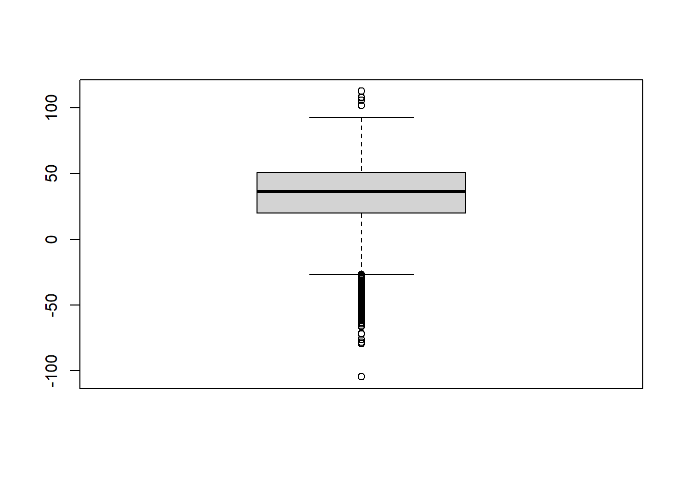

The average causal effect is the expected difference of the potential outcomes in the population of interest.

\[ACE = \mathbb{E}\left[Y^{a=1}\right] - \mathbb{E}\left[Y^{a=0}\right]\]

Estimate the average causal effect in the data and interpret your finding.

ACE_orcl = mean(ICE)
ACE_orcl

[1] 31.39465

Voilà! You just implemented your first estimator!

Intuitively, we estimated the average causal effect by the mean of the individual causal effects. \(\left(\hat{ACE}=\sum_{i=1}^n ICE_i\right)\). This was possible, because we assumed to know the counterfactuals for the individuals in the experiment. However, in reality we’d never observe both the treatment and non-treatment outcome for the same person. This is referred to as the fundamental problem of causal inference. Therefore, we call the estimator above oracle estimator.

So far, we have used the information on the counterfactuals that would usually not be available to us. Instead, let’s use a more realistic approach that is based on assumptions. Let’s assume that the experiment has been conducted properly so that the assumption of exchangeability or unconfoundedness was satisfied. If this is the case, we can estimate the average causal effect from the difference in the means of the observed outcome \(Y\) for the two treatment groups. Let’s do this next.

First of all, we construct the observed outcome from the potential outcomes in combination with the observed treatment assignment, i.e., \[Y = A \cdot Y^{a=1} + (1-A) \cdot Y^{a=0}\]

# calculate obs outcomes first outcome and attach it to the data frame
df$Y = df$A * df$Y_a1 + (1-df$A) * df$Y_a0

Now let’s use the difference in the conditional average of the outcome variable in both subgroups as an estimator for the average treatment effect.

ACE_obs = mean(df$Y[df$A == 1]) - mean(df$Y[df$A == 0])
ACE_obs

[1] 31.29618

We can observe that this empirical estimator is very close to the oracle estimator.

2 Simulation Study

A simulation is the imitation of the operation of a real-world process or system over time. Statisticians use simulation studies to empirically investigate the properties of their estimators. The key idea is to repeatedly generate data from the same DGP and re-run the estimator over and over again. Doing so, we gather many estimates and can look at the distributions of them. The distribution tells us more about bias and variance of the estimator. We can also measure and compare the performance of different estimators, for examples, based on the mean-squared error (w.r.t. to the true causal effect), the empirical coverage or the width of confidence intervals.

Let’s get more into the idea of a DGP. What would have happened if the treatment assignment was different in the example from Section 1? Use the R function sample() to generate a new realization of a random treatment assignment. Keep the probability to be treated \(P(A=1)\) at the same value as before.

# to make the code reproducible, use a seed
set.seed(1234)

# calculate observed treatment assignment probability
p <- sum(df$A == 1)/n

# assign new treatment at random with p
Z <- sample(c(0,1), size = n, replace = TRUE, prob = c(1-p, p))

# find a new realized outcome for each individual
Y2 <- Z*df$Y_a1 + (1-Z)*df$Y_a0

So, we drew a new sample, with \(p=\) 72.31 \(\%\) of the units being treated. Y2 are our new realized outcomes, based on which we can now run our estimator for the \(ACE\) again.

ACE_obs2 <- mean(Y2[Z==1]) - mean(Y2[Z==0])
ACE_obs2

[1] 30.19125

As expected, we get another estimate, which is neither identical to the first estimate nor to the oracle. This time, we are a little bit further off, with a bias of around 1.2. To make this a bit more systematic, run a small simulation study with \(R=100\) repetitions.

Whenever we want to use the same piece of code over and over again, it makes sense to encapsulate it in a function. Hence let us first define a function ate_obs(Y, Z) that performs the estimation of the ATE based on the conditional means of \(Y\) given treatment \(Z\).

ate_obs = function(Y, Z) {
  ACE = mean(Y[Z==1]) - mean(Y[Z==0])
  return(ACE)
}

We repeat the random assignment of the treatment 100 times and, every time we do so, we calculate the causal effect based on the observed outcomes. To implement this iterative execution, we set up a for-loop with \(R=100\) repetitions. We store the resulting estimates in a numeric vector, that we initialize before running the code in the for-loop.

# to make the code reproducible, use a seed
set.seed(1234)

# number of repetitions
R = 100

# vector for storing the individual estimates
ACEs <- rep(0, R)

# loop over all repetitions
for (i in 1:R){
  # assign new treatment as above
  this_Z <- sample(c(0,1), size = n, replace = TRUE, prob = c(1-p, p))
  
  # calculate the new realized outcome
  this_Y <- this_Z*df$Y_a1 + (1-this_Z)*df$Y_a0
  
  # estimate the ACE and store it in the prepared vector
  ACEs[i] <- ate_obs(this_Y, this_Z)
}

Let’s have a look on the empirical estimators.

# the head() function shows the first few results
head(ACEs)

[1] 30.19125 30.49999 31.83401 31.90579 30.72405 31.52555

Once again, we can generate a boxplot illustrate the simulation results. To compare the empirical estimators to the oracle estimator, we add a red horizontal line at the oracle value.

boxplot(ACEs)
abline(h = ACE_orcl, col = "red")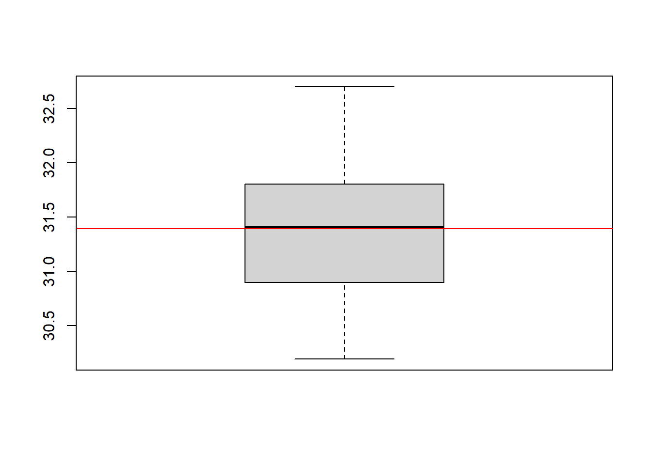

You can see, the median (solid line inside the boxplot) of our estimators is pretty close to the true value, which can be interpreted as evidence that our estimator is unbiased.

Whenever we observe that the the sample estimator differs from the population value in our example, this deviation can be entirely explained by the randomness that is inherent to the estimator. To be more precise, the randomness in our simulation study only arises due to a different treatment assignment, which in turn leads to a different realization of the observed outcomes and subsequently to a different value for the means in observed outcomes in the treatment groups.

3 IPW and Standardization

Let’s continue with a second example that is concerned with estimation of the average treatment effect in the presence of a confounder. We will see that in such a setting, the estimator from Section 1 will not consistently estimate the true causal effect. To address confounding, we have to adjust our estimation strategy and implement different estimators.

Load the data set experiment_data_counterfactual_Ex4.rda and find out the sample size and the oracle estimator for the average causal effect. The data frame is again called df. You find the counterfactual outcomes in the columns Y_a1 and Y_a0. The actual observed treatment is in the column A.

# load new data frame from URL
load(url("https://digitalcausalitylab.github.io/tutorial/intro_to_causal_inf/data/experiment_data_counterfactual_Ex4.rda"))

# number of observations
n <- dim(df)[1]
n

[1] 1919

# oracle eastimator for the ACE
ICE <- df$Y_a1 - df$Y_a0
ACE_orcl <- mean(ICE)
ACE_orcl

[1] 0.3272538

Add column Y for the realized outcome to the data frame.

# add realized outcome as a column
df$Y = df$A*df$Y_a1 + (1-df$A)*df$Y_a0

Below you find the code that reproduces this DGP in a simulation study with 250 observations. Again, we compute the estimator from above to estimate the ACE from the observed outcomes. We draw a boxplot of the estimates, which also includes the oracle estimator. What do you observe?

# set seed for reproducibility
set.seed(1234)

# calculate probability to be treated as observed in strata of L
n_l1 <- sum(df$L==1)
n_l0 <- sum(df$L==0)
p_l1 <- sum(df$A==1 & df$L==1)/n_l1
p_l0 <- sum(df$A==1 & df$L==0)/n_l0

# number of repetitions
R = 250

# vector for storing the individual estimates
ACEs <- rep(0, R)

# vector for storing the treatment assignment
this_Z <- rep(0, n)

# loop over all repetitions
for (i in 1:R){
  
  # new treatment assignment depending on value for L
  this_Z[df$L==1] <- sample(c(0,1), size = n_l1, replace = TRUE, prob = c(1-p_l1, p_l1))
  this_Z[df$L==0] <- sample(c(0,1), size = n_l0, replace = TRUE, prob = c(1-p_l0, p_l0))
  
  # new realized outcome
  this_Y <- this_Z*df$Y_a1 + (1-this_Z)*df$Y_a0
  
  # Estimate the ACE and store it in the prepared vector
  ACEs[i] <- ate_obs(this_Y, this_Z)
}

boxplot(ACEs, ylim=c(0.32,0.42))
abline(a = ACE_orcl, b = 0, col = "red")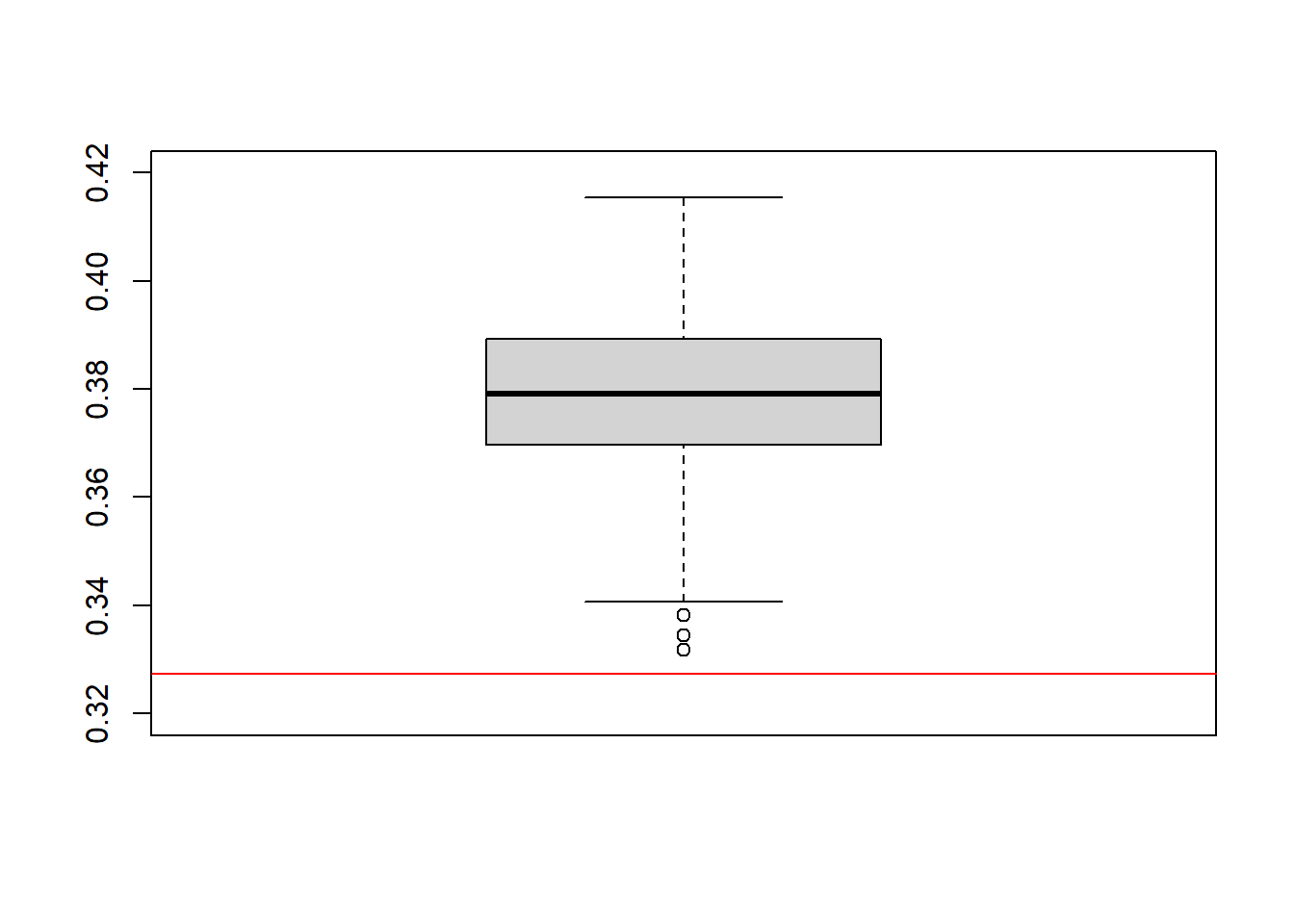

The results for this estimator don’t look too good. We observe an absolute bias of 0.05, on average. The deviation of the estimates from the true ACE seems to be systematic as it can no longer be attributed solely to estimation randomness. This is, as you might already figured out by yourself, because exchangeability does not hold in this DGP. The new data comes in strata \(L \in [0,1]\) which have a different treatment probabilities.

To show this, calculate the probability of being treated in each stratum.

p_l1 <- sum(df$A==1 & df$L==1)/n_l1
p_l0 <- sum(df$A==1 & df$L==0)/n_l0
print(paste("P(A=1 | L=0) = ", round(p_l0, 2)))

[1] "P(A=1 | L=0) =  0.32"

print(paste("P(A=1 | L=1) = ", round(p_l1, 2)))

[1] "P(A=1 | L=1) =  0.61"

We can use the counterfactual information to find out more about the confounding variable \(L\). As we have already seen from the difference in the probability to be treated, \(L\) has a causal effect on \(A\). Let’s find out if \(L\) also causally effects \(Y\). For each stratum of \(L\), we consider the difference in potential outcomes, which amounts to the Causal Risk Differences (CRD) in each subsample.

# causal risk difference (CRD) for L==1
CRD_l1 <- mean(df$Y_a1[df$L==1]) - mean(df$Y_a0[df$L==1])
CRD_l1

[1] 0.2909535

# CRD for L==0
CRD_l0 <- mean(df$Y_a1[df$L==0]) - mean(df$Y_a0[df$L==0])
CRD_l0

[1] 0.3916185

Hence, we can conclude that \(L\) has a causal effect on \(Y\), too. \(L\) is a confounder which we have to account for in our subsequent analysis.

As stated above, ACE_obs would consistently estimate the true ACE only if (unconditional) exchangeability held in the data generating process. However, this is not true in this example due to selection into treatment in terms of \(L\).

In the lecture you learned the methods of Inverse Probability Weighting (IPW) and standardization, which both account for a confounding variable \(L\). Implement the standardization estimator as a function and estimate the ACE based on the outcome variable \(Y\), the treatment variable \(A\) and the confounder \(L\).

standardization <- function(Y, A, L){
    n = length(Y)
    
    # ACE for Stratum: L=0
    PY_a1_l0 <- sum(Y[A==1 & L==0]==1)/length(Y[A==1 & L==0])
    PY_a0_l0 <- sum(Y[A==0 & L==0]==1)/length(Y[A==0 & L==0])
    ACE_obs_l0 <- PY_a1_l0 - PY_a0_l0
    
    # ACE for Stratum: L=1
    PY_a1_l1 <- sum(Y[A==1 & L==1]==1)/length(Y[A==1 & L==1])
    PY_a0_l1 <- sum(Y[A==0 & L==1]==1)/length(Y[A==0 & L==1])
    ACE_obs_l1 <- PY_a1_l1 - PY_a0_l1
        
    # return standartized ACE
    ACE_obs_std <- sum(L==1)/n * ACE_obs_l1 + (1-sum(L==1)/n) * ACE_obs_l0
    return(ACE_obs_std)
}

ACE_obs_std  <- standardization(df$Y, df$A, df$L)
ACE_obs_std

[1] 0.3973981

Now, implement the IPW estimator and also estimate the ACE and interpret your result.

IPW <- function(Y, A, L){
    n <- length(Y)
    
    # Branch 1: L=0
    f_a1_l0 <- sum(A==1 & L==0)/sum(L==0)
    f_a0_l0 <- sum(A==0 & L==0)/sum(L==0)

    # Branch 2: L=1
    f_a1_l1 <- sum(A==1 & L==1)/sum(L==1)
    f_a0_l1 <- sum(A==0 & L==1)/sum(L==1)

    weight_A1 <- (1-L)*f_a1_l0 + L*f_a1_l1
    PY_a1 <- 1/n * sum(Y*A/weight_A1)

    weight_A0 <- (1-L)*f_a0_l0 + L*f_a0_l1
    PY_a0 <- 1/n * sum(Y*(1-A)/weight_A0)

    ACE_obs_IPW <- PY_a1 - PY_a0
    return(ACE_obs_IPW)
}

ACE_obs_IPW <- IPW(df$Y, df$A, df$L)
ACE_obs_IPW

[1] 0.3973981

The estimate of the IPW estimator is equal to the estimate of the standardization estimator. Is this at random? Set up one final simulation study in which you compare the observational, the IPW and the standardization estimator for the ACE.

# set seed for reproducability
set.seed(1234)

# new probability to be treated as observed
n_l1 <- sum(df$L==1)
n_l0 <- sum(df$L==0)
p_l1 <- sum(df$A==1 & df$L==1)/n_l1
p_l0 <- sum(df$A==1 & df$L==0)/n_l0

# number of repetitions
R = 250

# vector for storing the individual estimates
ACEs_obs <- ACEs_std <- ACEs_IPW <- rep(0, R)

# vector for storing the treatment assignment
this_Z <- rep(0, n)

# loop over all repetitions
for (i in 1:R){
    # new treatment assignment
    this_Z[df$L==1] <- sample(c(0,1), size = n_l1, replace = TRUE, prob = c(1-p_l1, p_l1))
    this_Z[df$L==0] <- sample(c(0,1), size = n_l0, replace = TRUE, prob = c(1-p_l0, p_l0))
    
    # new realized outcome
    this_Y <- this_Z*df$Y_a1 + (1-this_Z)*df$Y_a0
    
    ACEs_obs[i] <- ate_obs(this_Y, this_Z)
    ACEs_std[i] <- standardization(this_Y, this_Z, df$L)
    ACEs_IPW[i] <- IPW(this_Y, this_Z, df$L)
}

For visualization, we will use the package cumstats, which you have to install first

install.packages("cumstats")

library(cumstats)
plot(1:R, cummean(ACEs_obs), ylab = "Cumulative Mean of ACEs", xlab = "Simulation repetitions", ylim = c( min(cummean(ACEs_obs), cummean(ACEs_std), cummean(ACEs_IPW)), max(cummean(ACEs_obs), cummean(ACEs_std), cummean(ACEs_IPW))))
points(1:R, cummean(ACEs_std), col = "green")
points(1:R, cummean(ACEs_IPW), col = "blue")
abline(a = ACE_orcl, b = 0, col = "red")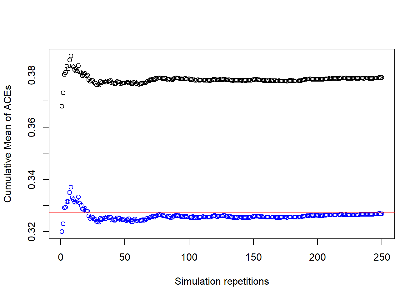

Figure 1: Cummulative mean of IPW and standardization estimates in simulation study. Red line indicates the oracle estimator (true effect).

This plot shows, that the standardization and IPW estimates are virtually identical and that both converge towards the oracle value of the estimate. Let’s have a look at the descriptive statistics for both estimates.

# Summary for IPW
summary(ACEs_IPW)

   Min. 1st Qu.  Median    Mean 3rd Qu.    Max. 
 0.2823  0.3161  0.3268  0.3269  0.3384  0.3682

# Summary for standardization
summary(ACEs_std)

   Min. 1st Qu.  Median    Mean 3rd Qu.    Max. 
 0.2823  0.3161  0.3268  0.3269  0.3384  0.3682

On average, the value is really close to the true causal effect. We can conclude from this evidence that both estimators are unbiased.

However, the estimator from Section 1, which does not take the variable \(L\) into account, converges to a different value, making it biased.

Another observation from the cumulative results in Figure 1 is that the cumulative mean of the estimates gets more and more stable and closer to the true value. This is because the more repetitions we have in our simulation, the smaller gets the variance of the estimates, on average.

4 Data Generating Processes and Directed Acyclic Graphs

In the examples above, we loaded a preprocessed data set that was generated outside our analysis. However, in many cases, it makes sense to provide our own implementation of a data generating process, i.e., in a function. To communicate your DGP, it is helpful to illustrate the DGP using a directed acyclic graph (DAG). We’ll see how we can use the R packages dagitty (Textor et al. 2016) and ggdag (Barrett 2022).

4.1 Setting up a DAG in R

Consider the following example: We want to implement a data generating process with a continuous treatment variable \(A\), a continous outcome variable \(Y\) and a (continuous) confounder \(L\) (similar to Section 3). We are interested in estimating the average treatment effect of \(A\) on \(Y\) taking the confounding by \(L\) into account. Such a DGP could be represented by the following DAG.

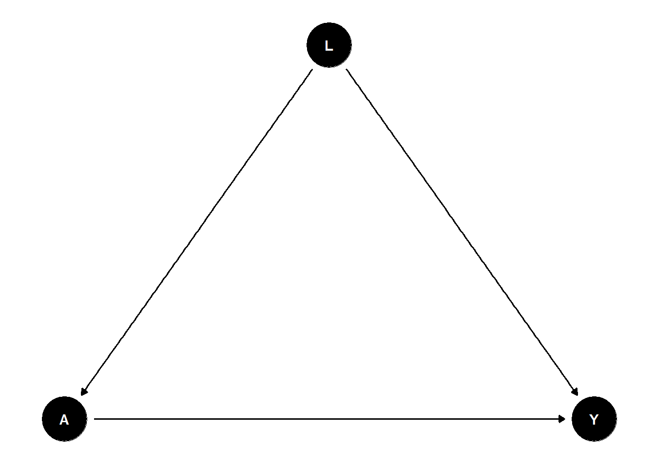
Hence, the DGP should include the following causal effects:

\(A \rightarrow Y\),
\(L \rightarrow A\),
\(L \rightarrow Y\).

For simplicity, we assume that the variables \(A\) and \(L\) are standard normal random variables. Moreover, we assume that the causal effects described in 1.-3. are linear and additive. We set the value of all (true) causal effects in our model to 1. In our regression specifications we also include a constant. Hence, we can implement the first causal effect (see 1.) as

4.2 Simulating Data based on a DAG

# set number of observations
n <- 1000

L <- rnorm(n, 0, 1)
A <- 0.5 + 1*L + rnorm(n, 0, 1)

Let’s now estimate the causal effect \(L\) has on \(A\) using a linear regression via lm().

lm(A ~ L)


Call:
lm(formula = A ~ L)

Coefficients:
(Intercept)            L  
     0.5140       0.9851

We can proceed in this way and encapsulate our DGP in a function DGP_confound(), which takes the number of observations as an argument and returns a data frame.

DGP_confound <- function(n) {
  L <- rnorm(n, 0, 1)
  A <- 0.5 + 1 * L + rnorm(n, 0, 1)
  Y <- 1 + 1 * A + 1 * L + rnorm(n, 0, 1)
  
  df <- data.frame(Y, A, L)
  return(df)
}

Let’s test whether the function really implements the DGP we wanted. Provided \(L\) is a confounder we expect to observe the following empirical results.

The coefficient of \(A\) in a linear regression of \(Y\) on \(A\) (i.e., excluding \(L\)) will not be an unbiased estimate for the true average treatment effect, which has a value of 1.
The coefficient of \(A\) in a linear regression of \(Y\) on \(A\) and \(L\) will will be an unbiased estimate for the true average treatment effect, which has a vaue of 1.

We generate one realization of the DGP above and test these two hypotheses using a corresponding linear regression model.

df <- DGP_confound(1000)

# Estimate linear regression of Y on A
reg_Y_A <- lm(Y ~ A, data = df)

# Estimate linear regression of Y on A **and** L
reg_Y_A_L <- lm(Y ~ A + L, data = df)

# Summarize regression output
summary(reg_Y_A)


Call:
lm(formula = Y ~ A, data = df)

Residuals:
    Min      1Q  Median      3Q     Max 
-4.4413 -0.8346  0.0216  0.8696  4.0692 

Coefficients:
            Estimate Std. Error t value Pr(>|t|)    
(Intercept)  0.74495    0.04201   17.73   <2e-16 ***
A            1.47346    0.02848   51.74   <2e-16 ***
---
Signif. codes:  0 '***' 0.001 '**' 0.01 '*' 0.05 '.' 0.1 ' ' 1

Residual standard error: 1.246 on 998 degrees of freedom
Multiple R-squared:  0.7285,    Adjusted R-squared:  0.7282 
F-statistic:  2677 on 1 and 998 DF,  p-value: < 2.2e-16

summary(reg_Y_A_L)


Call:
lm(formula = Y ~ A + L, data = df)

Residuals:
    Min      1Q  Median      3Q     Max 
-3.3758 -0.6993  0.0213  0.7183  3.5070 

Coefficients:
            Estimate Std. Error t value Pr(>|t|)    
(Intercept)  1.02510    0.03689   27.79   <2e-16 ***
A            0.98733    0.03235   30.52   <2e-16 ***
L            1.00119    0.04590   21.81   <2e-16 ***
---
Signif. codes:  0 '***' 0.001 '**' 0.01 '*' 0.05 '.' 0.1 ' ' 1

Residual standard error: 1.026 on 997 degrees of freedom
Multiple R-squared:  0.8162,    Adjusted R-squared:  0.8158 
F-statistic:  2213 on 2 and 997 DF,  p-value: < 2.2e-16

The regression output reveals that the linear regression of \(Y\) on \(A\) only leads to an omitted variable bias in the coefficient of \(A\). If we additionally include the confounder \(L\) in our regression analysis, the estimated effect is very close to the true effect with a value of 1.

Now it’s your turn!

In our function DGP_confound(n), we set the value for the causal effect of \(A\) on \(Y\) to a value of 1. Now, modify the implementation of DGP_confound(n, ce) such that the user can provide a value for the causal effect of \(A\) on \(Y\) through an argument ce.

In the next step, we will see how we can illustrate this DGP with a DAG.

First, we have to install the R packages dagitty and ggdag and load them afterwards.

install.packages("dagitty")
install.packages("ggdag")

library(dagitty)
library(ggdag)

We can generate a DAG with dagitty by specifying the DAG’s edges and nodes. In our example, the corresponding code would be

dag_confound <- dagitty("dag {
  Y <- A ;
  Y <- L ;
  A <- L ;
  }
")

We can print the DAG using print() or plot it using plot().

print(dag_confound)

dag {
A
L
Y
A -> Y
L -> A
L -> Y
}

plot(dag_confound)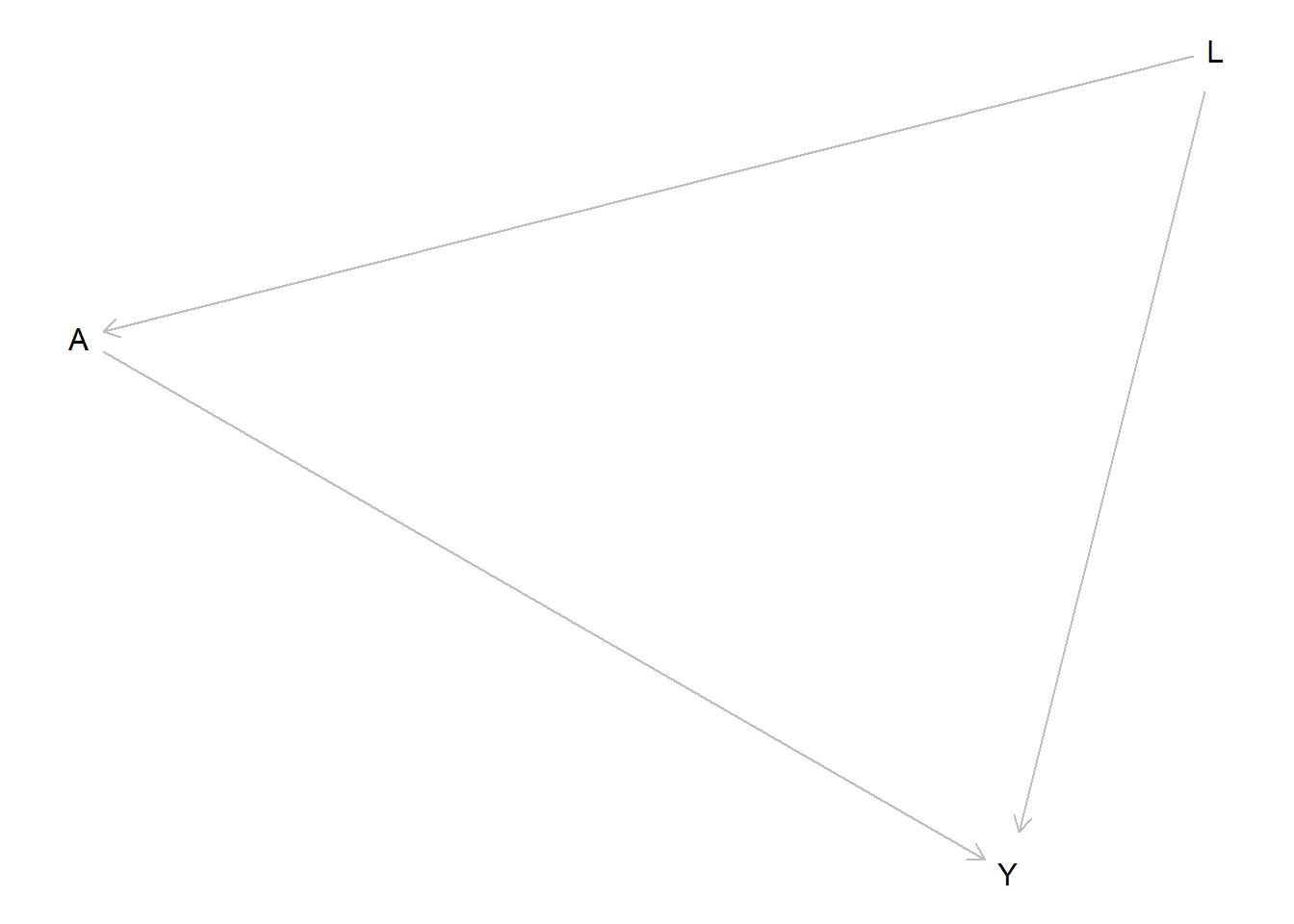

The package ggdag provides additional tools to work with DAGs which can be used to improve the visualization of the DAG. To work on our DAG, we use the function tidy_dagitty().

dag_confound_tidy <- tidy_dagitty(dag_confound)

The tidy DAG can now be plotted using ggdag().

ggdag(dag_confound_tidy)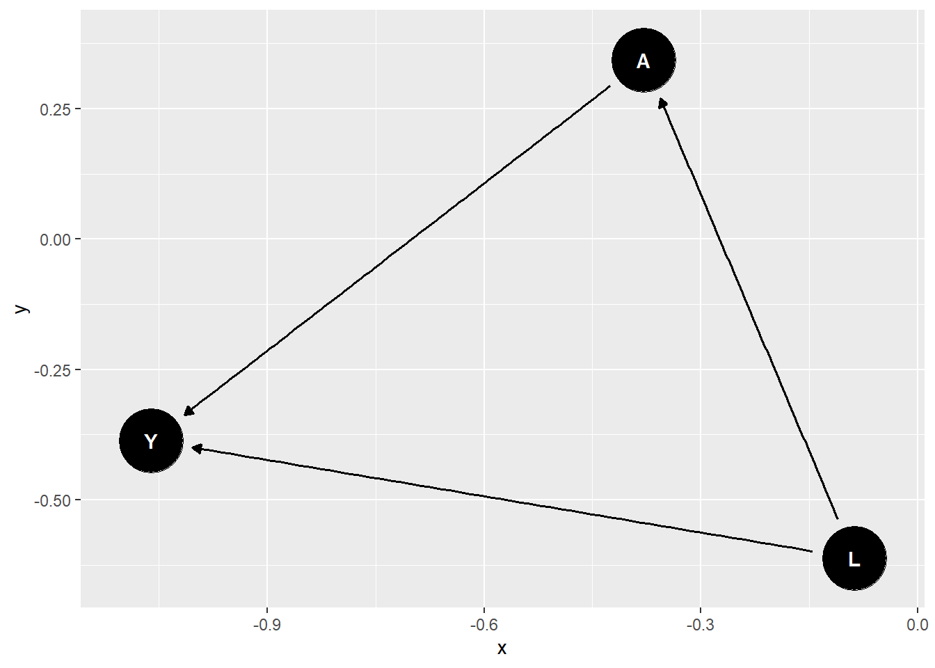

We can now set additional parameters with ggdag, for example a theme.

ggdag(dag_confound_tidy) + theme_dag_blank()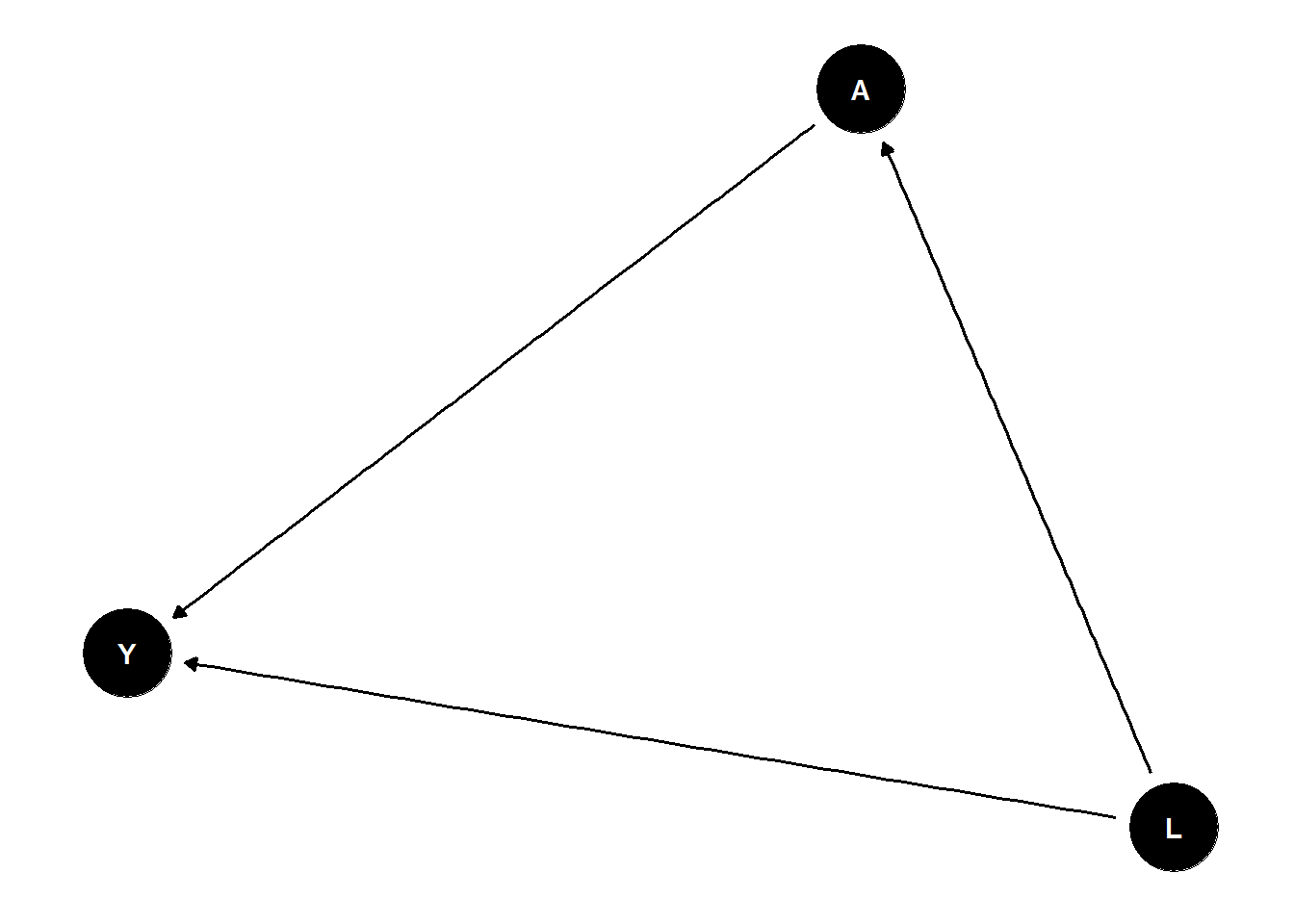

As an alternative to generating the DAG with dagitty first and converting it to ggdag is to directly generate the DAG with ggdag. It is possible to use another syntax there which is similar to the one that we used in lm() before.

dag_confound_ggdag <- dagify(
  Y ~ L + A,
  A ~ L
)

# Plot the DAG
ggdag(dag_confound_ggdag) + theme_dag_blank()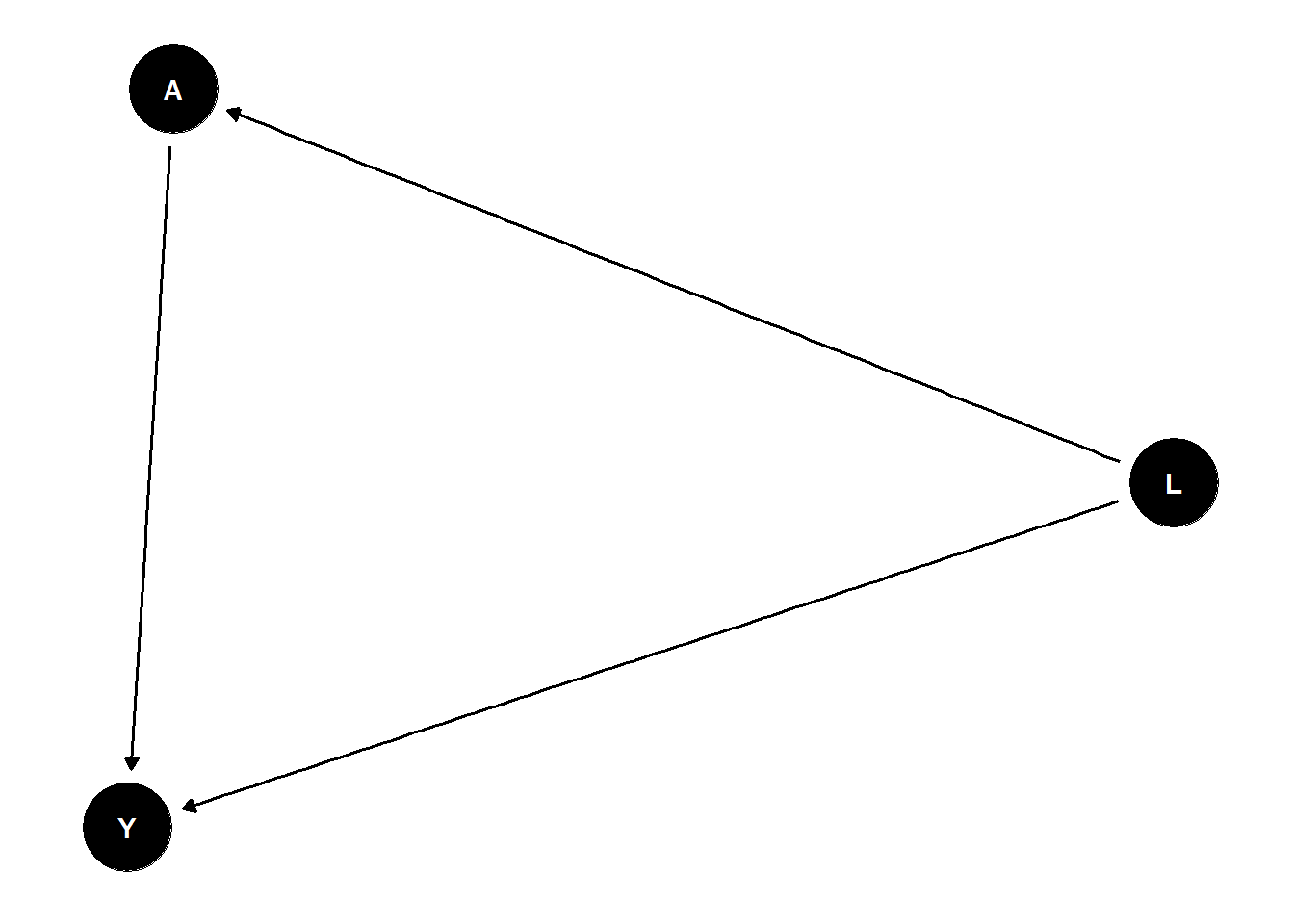

Finally, we can set some coordinates to modify the DAG.

dag_confound_ggdag <- dagify(
  Y ~ L + A,
  A ~ L,
  coords = list(x = c(A = 1, L = 2, Y = 3),
                y = c(A = 1, L = 2, Y = 1))
)

# Plot the DAG
ggdag(dag_confound_ggdag) + theme_dag_blank()

Now it’s your turn!

Try to modify the DAG above by

including additional variables,
adding labels to the nodes of \(A\) (to be “treatment”), \(L\) (“confounder”) and \(Y\) (“outcome”).

4.3 Properties of DAGs

dagitty encodes many helpful properties of a DAG, which we can evaluate. For example, we can find the parents, ancestors, children and descendants of a specific node.

Lets consider a bit more complicated example as of Figure 2.6. Glymour, Pearl, and Jewell (2016) . This example is based on this tutorial.

fig2.5 <- dagitty("dag {
    X -> R -> S -> T <- U <- V -> Y
}")
plot( graphLayout( fig2.5 ) )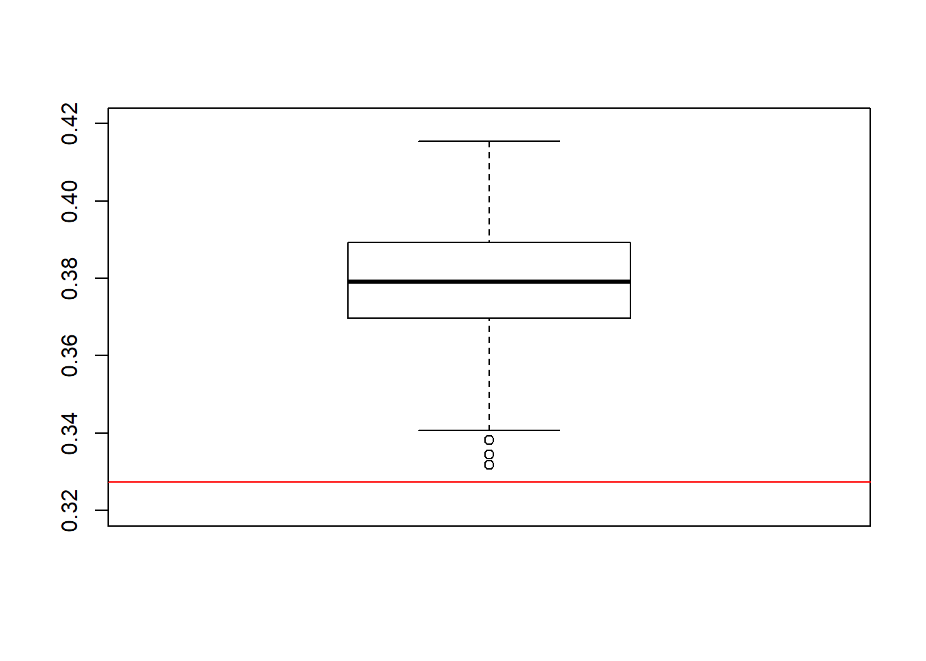

print(parents(fig2.5, "Y"))

[1] "V"

print(ancestors(fig2.5, "S"))

[1] "S" "R" "X"

print(children(fig2.5, "V"))

[1] "U" "Y"

print(descendants(fig2.5, "X"))

[1] "X" "R" "S" "T"

We can also output all paths between two variables.

paths(fig2.5, "Y", "S")$path

[1] "Y <- V -> U -> T <- S"

For example, we could list all pairs of variables in the graph that are independent conditional on the set \(Z = \{R, V\}\)

paths( fig2.5, "X", "Y", c("R","V") )

$paths
[1] "X -> R -> S -> T <- U <- V -> Y"

$open
[1] FALSE

pairs <- combn( c("X","S","T","U","Y"), 2 )
apply( pairs, 2, function(x){
    p <- paths( fig2.5, x[1], x[2], c("R","V") )
    if( !p$open ){
        message( x[1]," and ",x[2]," are independent given {R,V}" )
    } else {
        message( x[1]," and ",x[2]," are possibly dependent given {R,V}" )
    }
} )

X and S are independent given {R,V}

X and T are independent given {R,V}

X and U are independent given {R,V}

X and Y are independent given {R,V}

S and T are possibly dependent given {R,V}

S and U are independent given {R,V}

S and Y are independent given {R,V}

T and U are possibly dependent given {R,V}

T and Y are independent given {R,V}

U and Y are independent given {R,V}

NULL

We can also print the implied conditional independencies in the DAG.

impliedConditionalIndependencies( fig2.5 )

R _||_ T | S
R _||_ U
R _||_ V
R _||_ Y
S _||_ U
S _||_ V
S _||_ X | R
S _||_ Y
T _||_ V | U
T _||_ X | R
T _||_ X | S
T _||_ Y | V
T _||_ Y | U
U _||_ X
U _||_ Y | V
V _||_ X
X _||_ Y

5 Conclusion

In this tutorial you learnt how to implement an estimator as a function in R, and how you can assess the empirical performance of the estimator in a simulation study. Moreover, you made your first steps to implement a DAG by yourself as well as illustrating a data generating process with the help of a DAG. You can find more resources on the R packages ggag and dagitty via the links provided in Section 6.

6 Helpful Resources

Tutorial on ggdag, https://ggdag.malco.io/articles/intro-to-ggdag.html
Resources on dagitty, http://www.dagitty.net/learn/index.html

References

Barrett, Malcom. 2022. Ggdag: Analyze and Create Elegant Directed Acyclic Graphs. https://cran.r-project.org/web/packages/ggdag/index.html.

Glymour, Madelyn, Judea Pearl, and Nicholas P Jewell. 2016. Causal Inference in Statistics: A Primer. John Wiley & Sons. http://bayes.cs.ucla.edu/PRIMER/.

Textor, Johannes, Benito van der Zander, Mark S. Gilthorpe, Maciej Liskiewicz, and George TH Ellison. 2016. “Robust Causal Inference Using Directed Acyclic Graphs: The r Package ’Dagitty’.” International Journal of Epidemiology 45: 1887–94.