Tutorial 1 - Recap: Statistics

Outline

Hernán and Robins (2020) summarize the probably most important question of causal inference as follows:

“The question is then under which conditions real world data can be used for causal inference”

In a particular situation (as in our case study example from the lecture), we want to know if a treatment $A$ has a causal impact on outcome $Y$. In practice, we cannot observe counterfactuals and have to live with data from randomized experiments. In many cases, even that is not possible and we have to work with observational data.

In any case, we need to use statistical tools to come up with an estimate of the average causal effect and thereby, need to have a good understanding of the assumptions that have to be satisfied to establish causality. This is why we will recap the basics of statistics in our first tutorial.

You may recap your notes from introductory statistics (“Statistik für Betriebswirte I & II”) to prepare the tutorial. Please, read the suggested additional reading as indicated on the last page of this problem set.

As this problem set is quite extensive, please do the following

• Recap the statistical concepts in Exercise 1 and Exercise 2
• Try to solve the following exercises on your own
  • Exercise 1, c), f), g)
  • Exercise 2, b), c), d)
  • Exercise 3

1 Exercise 1 - Probabilities

1. Define the requirements of a probability measure.

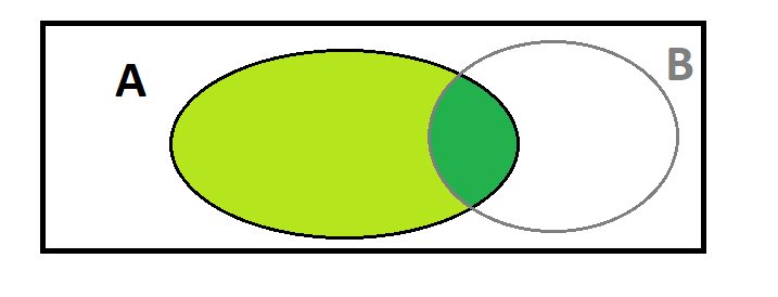
2. Provide the definition of the law of total probability. Draw a Venn diagram to illustrate the intuition behind it.

3. Write down Bayes’ rule to compute conditional probabilities.

4. Provide a definition of stochastic independence for events.

5. Define a random variable. What is the definition of stochastic independence for random variables? Can you provide examples of stochastically independent and stochastically dependent random variables?

6. Use Bayes’ rule to calculate the probability of being sick under a positive diagnosis and the probability of being healthy under a negative diagnosis in the following example

On average 2% of the population of a developing country have tuberculosis (tbc). If the disease is present, a tbc-diagnosis (d) is positive in 95% of the cases. However, if the disease is not present, 4% of the diagnoses are incorecctly declared as positive.

7. Consider Table 1 that shows the relationship between gender and education level in the U.S. Calculate the following probabilities using the law of total probability and Bayes’ rule
   • $P(\text{high school})$,
   • $P(\text{high school }OR\text{ female})$,
   • $P(\text{high school }|\text{ female})$,
   • $P(\text{female }|\text{ high school})$.

Note: You can assume, that the highest degree is meant here. You don’t need to include college graduated in your high school numbers.

Table 1: Frequency table, gender and educational achievement in the U.S.

Gender	Highest education achieved	Occurence (x 100.000)
Male	Never finished high school	112
Male	High school	231
Male	College	595
Male	Graduate School	242
Female	Never finished high school	136
Female	High school	189
Female	College	763
Female	Graduate School	172

2 Exercise 2 - Expected Values, Variance and Covariance

1. Provide the definition of

   • 1. the expected value of a discrete random variable $X$, $E(X)$,
   • 2. the expected value of a continuous random variable $X$, $E(X)$,
   • 3. the variance of a random variable $X$, $Var(X)$,
   • 4. the covariance of the random variables $X$ and $Y$, $Cov(X,Y)$,
   • 22. the correlation coefficient of two random variables $X$ and $Y$, ${\rho }_{X,Y}$.
         

2. Calculate $E(X)$, $E(Y)$ and $Var(X)$ for random variables $X$ and $Y$ with probability mass functions $f_X(X)$ and $f_Y(Y)$: $$\begin{array}{r}{f}_X(X)=\{\begin{array}{ll}& 1/3\text{ , if }x=0,\\ & 2/3\text{ , if }x=1,\\ & 0\text{ , otherwise }\end{array}.\end{array}$$ and $$\begin{array}{r}{f}_Y(Y)=\{\begin{array}{ll}& 1/6\text{ , if }y=0,\\ & 2/6\text{ , if }y=1,\\ & 3/6\text{ , if }y=2,\\ & 0\text{ , otherwise }\end{array}.\end{array}$$ Are these discrete or continuous random variables?

3. Consider the probabilities in Table 2 for additional random variables $X$ and $Y$ (values for $X$ depicted in rows, values for $Y$ in columns) and

   • 1. decide whether $X$ and $Y$ are stochastically independent,
   • 2. calculate $Cov(X,Y)$ and ${\rho }_{X,Y}$.

Table 2: Probability table for random variables $X$ (rows) and $Y$ (columns).

	1	3	10
2	0.05	0.03	0.02
4	0.20	0.10	0.05
6	0.20	0.25	0.10

4. Show that whenever $X$ and $Y$ are independent, then $Cov(X,Y)={\rho }_{X,Y}=0$.
   • Hint: Use $P_{X,Y}(X=x,Y=y)=P_X(X=x)\cdot P_Y(Y=y)$ to show that $E(X\cdot Y)=E(X)\cdot E(Y)$ under stochastic independence.

3 Exercise 3 - A Prior to Causality

It is important to keep in mind the difference between association and causality. Recalling the definition of causality, what seems wrong to you in the following examples?

1. “Data show that income and marriage have a high positive correlation. Therefore, your earnings will increase if you get married.”
2. “A study reports that there is a zero correlation between two variables $A$ and $Y$. Hence, there is no causal effect of $A$ on $Y$.”
3. “Data show that as the number of fires increase, so does the number of fire fighters. Therefore, to cut down on fires, you should reduce the number of fire fighters.”
4. “A study reports that there is a zero correlation between two variables $A$ and $Y$. Hence, $A$ and $Y$ are independent of each other.”
5. “Data show that people who hurry tend to be late to their meetings. Don’t hurry, or you’ll be late.”
6. “A study reports that there is a positive correlation between variables $A$ and $T$. Hence, $A$ has a causal effect on $Y$.”

4 Additional Reading

Parts of this tutorial are based on Chapter 1.3 of Glymour, Pearl, and Jewell (2016). You might read Chapter 1 completely to develop some intuition about the topic. A very accessible recap of probability and regression is also available in Chapter 2 of Cunningham (2021).

Cunningham, Scott. 2021. “Causal Inference.” In Causal Inference. Yale University Press. https://mixtape.scunning.com/.

Glymour, Madelyn, Judea Pearl, and Nicholas P Jewell. 2016. Causal Inference in Statistics: A Primer. John Wiley & Sons. http://bayes.cs.ucla.edu/PRIMER/.

Hernán, Miguel A, and James M Robins. 2020. “Causal Inference.” Boca Raton: Chapman & Hall/CRC. https://www.hsph.harvard.edu/miguel-hernan/causal-inference-book/.

5 Solution

5.1 Solution - Exercise 1

a. Probability measure

A probability measure $P$ on a sample space $\mathrm{\Omega }$ has to satisfy the following requirements (see Lecture Notes Introduction to Statistics (“Statistik 1”), p. 318).

1. For any event $A\subseteq \mathrm{\Omega }$ we have,
   • $P(A)\in [0,1]$
   • $P(\mathrm{\Omega })=1$
2. For countable events $A_1,A_2,\dots$ with $A_i\cap A_j=\mathrm{\varnothing }$ for $i\ne j$ we have
   • $P\left(\bigcup _{i=1}^{\mathrm{\infty }}{A}_i\right)=\sum _{i=1}^{\mathrm{\infty }}P(A_i).$

(This implies $P(\mathrm{\varnothing })=0$, since $\mathrm{\Omega }=\mathrm{\Omega }\cup \mathrm{\varnothing }\cup \mathrm{\varnothing }\dots$.)

Example 1: Toss a fair coin. Then $\mathrm{\Omega }=\{\text{"heads"},\text{"tails"}\}$. H denotes the event “heads” and T be the event “tails” with $P(H)=P(\text{"heads"})=0.5$ and $P(T)=P(\text{"tails"})=0.5$. Since $P(A\cap B)=0$, we have $P(A\cup B)=1$.

b. Definition of the law of total probability

• For mutually exclusive events $A$ and $B$ ($A\cap B=\mathrm{\varnothing }$), we always have $P(A\cup B)=P(A)+P(B)$.

• For any two events $A$ and $B$ we have $P(A)=P(A\cap B)+P(A\cap B^c)$ where $B^c$ denotes the complement of $B$ (“”).

• More generally, for any set of events $B_1,B_2,\cdots ,B_n$ such that exactly one of the events must be true (an exhaustive, mutually exclusive set, called a partition), we have $$P(A)=P(A\cap B_1)+P(A\cap B_2)+\cdots +P(A\cap B_n).$$ Finally, the Law of Total Probability states $$P(A)=P(A|B_1)P(B_1)+P(A|B_2)P(B_2)+\cdots +P(A|B_n)P(B_n)$$ using the Bayes’ Rule.

Illustration of Law of Total Probability (with n=2).

Illustration of Law of Total Probability (with n=8).

c. Bayes’ rule

• For two events $A$ and $B$, Bayes’ rule states that

$$P(A|B)=\frac{P(A\cap B)}{P(B)}=\frac{P(B|A)P(A)}{P(B)}.$$

• More events: Let $A_1,\dots ,A_N$ be a partition of $\mathrm{\Omega }$. Bayes’ rule implies

$$P(A_i|B)=\frac{P(B|A_i)P(A_i)}{P(B)}=\frac{P(B|A_i)P(A_i)}{\sum _{j=1}^{N}P(B|A_j)P(A_j)}.$$

d. Stochastic independence

• Two events $A$ and $B$ are said to be independent if

$$P(A\cap B)=P(A)\cdot P(B).$$

Or, equivalently (simply plug the previous definition into Bayes’ rule)

$$P(A|B)=P(A).$$

• In Example 1, are the events H and T stochastically independent?

• Further, two events $A$ and $B$ are conditionally independent given a third event $C$ if $$P(A|B,C)=P(A|C).$$

• Note: $A$ and $B$ are called marginally independent if the the statement holds without conditioning on $C$.

e. Random variables

Let $(\mathrm{\Omega },P)$ be a probability space. A real-valued random variable $X$ is a measurable function $X:\mathrm{\Omega }\to \mathbb{R}$.

• Two random variables $Y$ and $X$ are said to be independent of each other if for every value $y$ and $x$ that $Y$ and $X$ can take we have $$P(X=x|Y=y)=P(X=x).$$

• Whenever $X$ and $Y$ are independent, we have that the joint probability function/density is equal to the product of marginal probability functions/densities $$P_{X,Y}(X=x,Y=y)=P_X(X=x)\cdot P_Y(Y=y)$$ for all $x,y$ for discrete random variables and $$f_{X,Y}(x,y)=f_X(x)\cdot f_Y(y)$$ for continuous random variables.

Example 2: Let us consider two independent coin flips (similiar to example 1). Let $X$ denote the output of the first coin flip, $Y$ denotes the output of our second coin flip. Then $X$ and $Y$ are stochastically independent.

Example 3: Assume that we are rolling a fair dice. Let $X$ denote the output of this experiment. Hence, $X$ takes values $1,2,\dots ,6$. $Y$ indicates if the number is even. Hence, $Y$ takes the value $1$ (even) or $0$ (odd). Then $X$ and $Y$ are stochastically dependent. Why?

f. Application of Bayes’ rule

• The given probabilities are $$\begin{array}{rl}P(tb{c}^{+})=0.02& \Rightarrow P(tb{c}^{-})=0.98\\ P(d^{+}|tb{c}^{+})=0.95& \Rightarrow P(d^{-}|tb{c}^{+})=0.05\\ P(d^{+}|tb{c}^{-})=0.04& \Rightarrow P(d^{-}|tb{c}^{-})=0.96.\end{array}$$

Therefore we have $$\begin{array}{rl}P(tb{c}^{+}|d^{+})& =\frac{P(d^{+}|tb{c}^{+})P(tb{c}^{+})}{P(d^{+}|tb{c}^{+})P(tb{c}^{+})+P(d^{+}|tb{c}^{-})P(tb{c}^{-})}\\ & =\frac{0.95\cdot 0.02}{0.95\cdot 0.02+0.04\cdot 0.98}\approx 32.6.\mathrm{\%}\\ P(tb{c}^{-}|d^{-})& =\frac{P(d^{-}|tb{c}^{-})P(tb{c}^{-})}{P(d^{-}|tb{c}^{-})P(tb{c}^{-})+P(d^{-}|tb{c}^{+})P(tb{c}^{+})}\\ & =\frac{0.96\cdot 0.98}{0.96\cdot 0.98+0.05\cdot 0.02}\approx 99.9.\mathrm{\%}.\end{array}$$

g. Gender and education example

• We start by adding the sum of occurrences to the table to calculate the number of individuals.

Gender	Highest education achieved	Occurence (x 100.000)
Male	Never finished high school	112
Male	High school	231
Male	College	595
Male	Graduate School	242
Female	Never finished high school	136
Female	High school	189
Female	College	763
Female	Graduate School	172
.	.	2440

• It may be helpful to represent the frequencies in a contingency table. Our variables of interest are female and high school.

Contingency table, absolute frequencies.

	High school	No high school	Sum
Male	231	949	1180
Female	189	1071	1260
Sum	420	2020	2440

Contingency table, relative frequencies.

	High school	No high school	Sum
Male	0.0947	0.3889	0.4836
Female	0.0775	0.4389	0.5164
Sum	0.1721	0.8279	1.0000

• Let $H$ denote the event “a person has highest education achieved high school” and $F$ denote the event “a person is female”. Then we can calculate, $$P(\text{high school})=P(H)=P(H\cap \overline{F})+P(H\cap F)=\frac{231}{2440}+\frac{189}{2440}=0.1721.$$

• We calculate $$\begin{array}{rl}P(\text{high school }OR\text{ female})& =P(H\cup F)\\ & =P(H)+P(F)-P(H\cap F)\\ & =\frac{420}{2440}+\frac{1260}{2440}-\frac{189}{2440}=\frac{1491}{2440}\\ & \approx 0.611\end{array}$$

• We use Bayes’ rule to calculate $$\begin{array}{rl}P(\text{high school }|\text{ female})& =\frac{P(H\cap F)}{P(F)}\\ & =\frac{189/2440}{1260/2440}=0.15.\end{array}$$

• We use Bayes’ rule to calculate $$\begin{array}{rl}P(\text{female }|\text{ high school})& =\frac{P(F\cap H)}{P(H)}\\ & =\frac{189/2440}{420/2440}=0.45.\end{array}$$

5.2 Solution - Exercise 2

a. Definitions

$$\begin{array}{r}E(X):=\sum _{x}x\cdot P(X=x)\end{array}$$ (discrete random variable) and $$\begin{array}{r}E(X):={\int }_{x}x\cdot f_X(X=x)dx\end{array}$$ (continuous random variable). $$\begin{array}{r}Var(X):=E((X-E(X){)}^2)=E(X^2)-E(X{)}^2(=\sum _x{x}^2\cdot P(X=x)-{(\sum _{x}x\cdot P(X=x))}^2).\end{array}$$

$$\begin{array}{rl}Cov(X,Y)& =E(X,Y)-E(X)\cdot E(Y).\end{array}$$

$$\begin{array}{r}{\rho }_{x,y}=\frac{Cov(X,Y)}{\sqrt{Var(X)\cdot Var(Y)}}.\end{array}$$

b. Expectations and variance

Calculate $E(X)$, $E(Y)$ and $Var(X)$ for the random variables $X$ and $Y$ with probability mass functions $f_X(X)$ and $f_Y(Y)$: $$\begin{array}{r}{f}_X(X)=\{\begin{array}{ll}& 1/3\text{ , if }x=0,\\ & 2/3\text{ , if }x=1,\\ & 0\text{ , otherwise. }\end{array}\end{array}$$ and $$\begin{array}{r}{f}_Y(Y)=\{\begin{array}{ll}& 1/6\text{ , if }y=0,\\ & 2/6\text{ , if }y=1,\\ & 3/6\text{ , if }y=2,\\ & 0\text{ , otherwise .}\end{array}\end{array}$$

$$\begin{array}{rl}E(X)& =1/3\cdot 0+2/3\cdot 1=2/3(=P(X=1)).\end{array}$$

$$\begin{array}{rl}E(Y)& =1/6\cdot 0+2/6\cdot 1+3/6\cdot 2=2/6+6/6=4/3.\end{array}$$

$$\begin{array}{r}Var(X)=(1/3\cdot 0^2+2/3\cdot 1^2)-(2/3{)}^2=0.2222.\end{array}$$

c. Stochastic independence

Consider the following probability table showing the joint probability function for random variables $X$ and $Y$ and + i. decide whether $X$ and $Y$ are stochastically independent, + ii. calculate $Cov(X,Y)$ and ${\rho }_{X,Y}$.

Probability table (X: rows, Y: columns).

	1	3	10
2	0.05	0.03	0.02
4	0.20	0.10	0.05
6	0.20	0.25	0.10

• First we calculate the marginal probabilities of $X$ and $Y$

Marginal Distributions

	1	3	10	P(X=x)
2	0.05	0.03	0.02	0.10
4	0.20	0.10	0.05	0.35
6	0.20	0.25	0.10	0.55
P(Y=y)	0.45	0.38	0.17	1.00

• $X$ and $Y$ are not stochastically independent since, for instance, $P(X=2,Y=1)=0.05\ne 0.045=P(X=2)\cdot P(Y=1)$.

$$\begin{array}{rl}E(X)& =0.10\cdot 2+0.35\cdot 4+0.55\cdot 6=4.9,\\ E(Y)& =0.45\cdot 1+0.38\cdot 3+0.17\cdot 10=3.29.\end{array}$$

$$\begin{array}{rl}Var(X)& =0.10\cdot 2^2+0.35\cdot 4^2+0.55\cdot 6^2-{4.9}^2=25.8-{4.9}^2=1.79,\\ Var(Y)& =0.45\cdot 1+0.38\cdot 3+0.17\cdot 10-{3.29}^2=20.87-{3.29}^2=10.0459.\end{array}$$

$$\begin{array}{rl}Cov(X,Y)& =(2\cdot 1\cdot 0.05+....+6\cdot 10\cdot 0.10)-4.9\cdot 3.29\\ & =16.38-4.9\cdot 3.29=0.259.\end{array}$$

$$\begin{array}{rl}{\rho }_{X,Y}& =\frac{0.259}{\sqrt{1.79\dot{1}0.0459}}=0.0610.\end{array}$$

The correlation between $X$ and $Y$ is very small.

d. Independence and correlation

Show that whenever $X$ and $Y$ are independent, then $Cov(X,Y)={\rho }_{X,Y}=0$.

Whenever $X$ and $Y$ are independent, we have that the joint probability is equal to the product of marginal probabilities $$P_{X,Y}(X=x,Y=y)=P_X(X=x)\cdot P_Y(Y=y).$$ It follows for

$$\begin{array}{rl}E(X\cdot Y)& =\sum _x\sum _{y}x\cdot y\cdot P_{X,Y}(X=x,Y=y)\\ & =\sum _x\sum _{y}x\cdot y\cdot P_X(X=x)\cdot P_Y(Y=y)\\ & =\sum _{x}x\cdot P_X(X=x)\sum _{y}y\cdot P_Y(Y=y)\\ & =E(X)\cdot E(Y).\end{array}$$

It follows immediately $Cov(X,Y)=E(X\cdot Y)-E(X)\cdot E(Y)=E(X)\cdot E(Y)-E(X)\cdot E(Y)=0$.